Background

This was my first task when I started working on Titus excutor. Since it was also the first time I worked on SQL performance issues, I think it’s worth noting it down for future reference.

One component of Titus executor is called Titus VPC Service, which is responsible for allocating IP addresses for Titus containers. In Titus VPC Service, there is a complex SQL query that involves several table joins. It looks like the following (adapted to use specific query parameters):

SELECT COUNT(*)
FROM branch_eni_attachments
JOIN branch_enis ON branch_enis.branch_eni = branch_eni_attachments.branch_eni
JOIN trunk_enis ON branch_eni_attachments.trunk_eni = trunk_enis.trunk_eni
JOIN availability_zones ON trunk_enis.account_id = availability_zones.account_id
AND trunk_enis.az = availability_zones.zone_name
WHERE branch_eni_attachments.association_id NOT IN (SELECT branch_eni_association FROM assignments)
    AND branch_eni_attachments.attachment_completed_at < now() - (60 * interval '1 sec')
    AND branch_eni_attachments.state = 'attached'
    AND branch_enis.last_used < now() - (3600 * interval '1 sec')
        AND branch_enis.subnet_id = 'subnet-1a391a47';

The database engine is PostgreSQL.

Problem

Without any code changes, the execution time of this query suddenly increased from a couple hundreds of milliseconds to 7+ minutes on one day!

This PR, which changed the NOT IN clause to NOT EXISTS, seemed to make the issue disappear. However, my curiosity wasn’t satisfied because of the following unanswered questions:

• According to this Stackoverflow answer, NOT IN and NOT EXIST will have performance difference when NULLs are allowed on the column. However, the column in this query is not nullable.
• Even if they NOT IN and NOT EXIST indeed have huge performance difference, then why suddenly the issue started on one day rather than since day one?

In order to satisfy my curiosity, I ran the following analysis.

Analysis

Background: Query Execution Plan

A query execution plan is how a query is executed by the database. Just like there are different ways of writing code to implement the same functionality, there are different ways to execute a SQL query. Because of that, comparing “NOT IN” query with “NOT EXIST” query and saying one is faster or slower than the other is not accurate.

What’s more important is the query execution plan, which can be evaluated by using EXPLAIN. With different query execution plans and different execution runtime (e.g. how many rows are returned in each node of the execution plan. I’ll cover “node” later), it’s entirely possible that:

• A NOT IN query is much faster than its NOT EXIST equivalent.
• A NOT IN query is much slower than its NOT EXIST equivalent.
• When the same query is executed with different plans, one is significantly faster or slower than the other.

In short, changing from NOT IN to NOT EXIST fixed the problem not because the latter is always faster than the former but because it changed the execution plan selection of Postgres query planner.

Query Execution Plan during the Incident

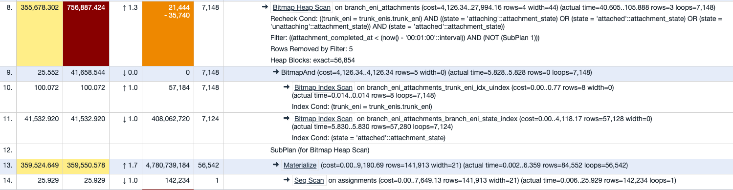
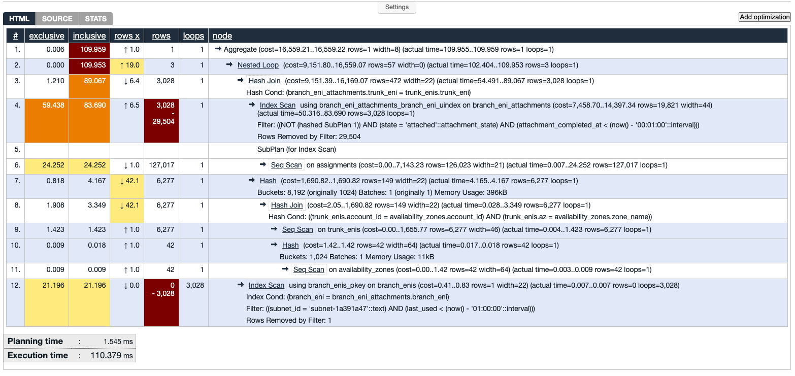
It took me quite some time to try to (fail to) reproduce the slowness. Running the old NOT IN query takes less than 1 second now and is even faster than the equivalent NOT EXIST query. Thankfully, a colleague of mine saved an output of EXPLAIN ANALYZE on the day of the issue. Copying the graph here:

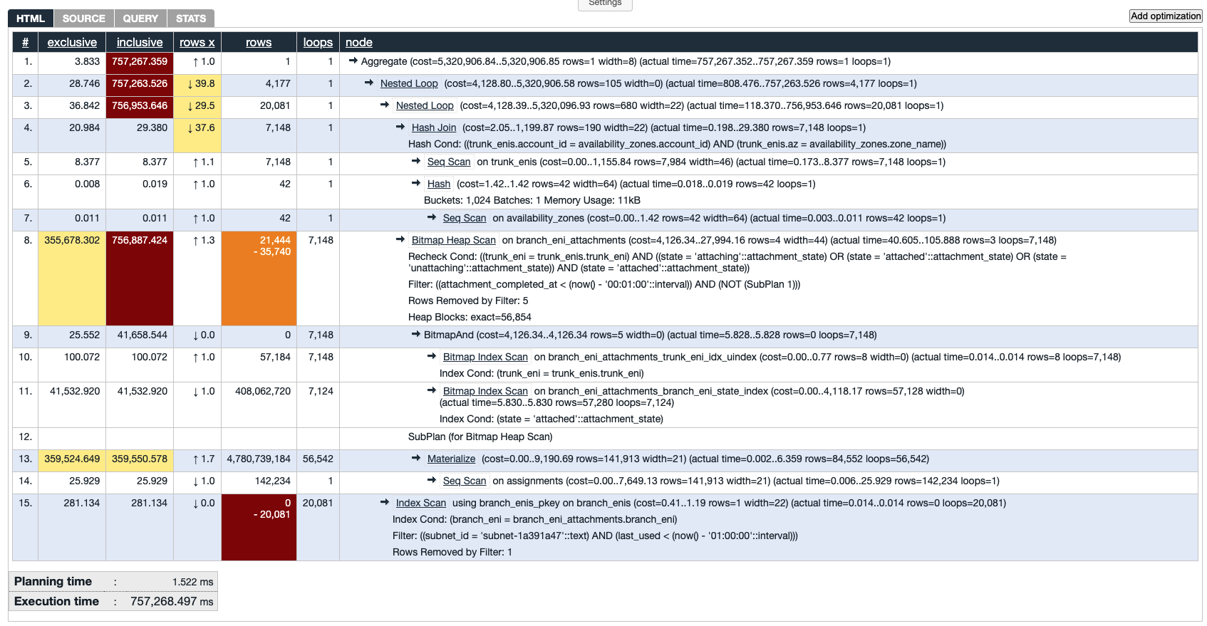
The next question is, why is this query plan extremely slow? To answer this question, we need to understand the query first. Personally, I find it’s easier to understand the execution plan by converting it to the equivalent pseudo-code. I’ll do the conversion step by step.

Convert to a Tree

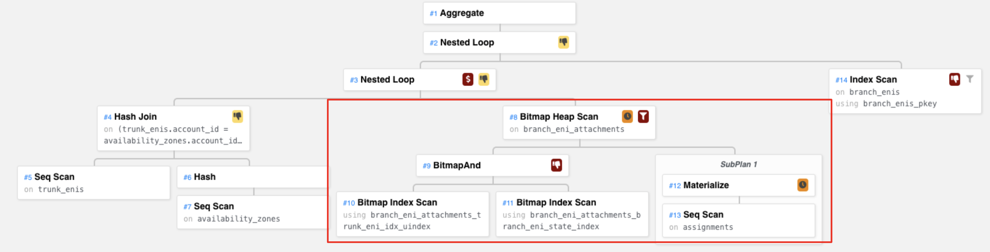
I find it easier to visualize the query plan using a tree structure. The query plan in a tree looks like this:

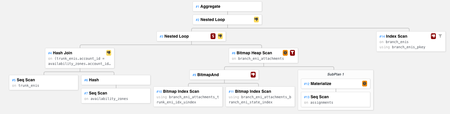
The diagram is generated by explain.dalibo.com.

Notes:

• Each node is an operation such as join, scan, etc.
• A parent node can only be executed after all child nodes are executed.
• Each node may be executed more than once (i.e. in a loop).

To better understand the operation of each node, I recommend reading [2] and [3].

Hash Join

First, let’s look at the Hash Join subtree.

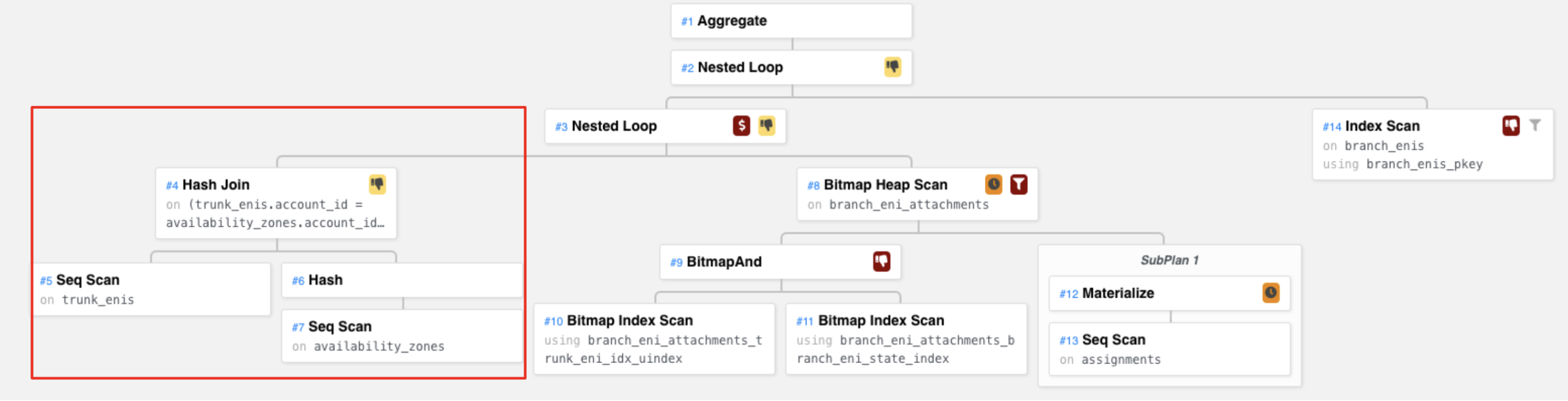
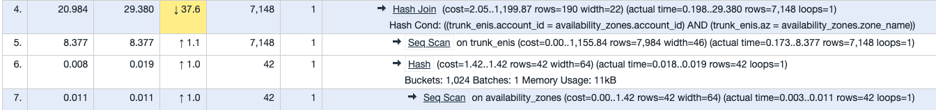
The corresponding query plan:

The pseudo code to explain this operation is

map<string, Az> az_by_account_id;
map<string, Az> az_by_zone_name;
for az in availability_zones // Seq Scan availability_zones
  az_by_account_id[hash(az.account_id)] = az // Hash
  az_by_zone_name[hash(az.zone_name)] = az   // Hash

for trunck_eni in trunk_enis // Seq Scan trunk_enis
  account_id_key = hash(trunk_eni.account_id)
  zone_name_key = hash(trunk_eni.az)
  // Hash Join
  if account_id_key in az_by_account_id && zone_name_key in az_by_zone_name
    return join(az_by_account_id[key], trunk_eni)

According to the query EXPLAIN result, this Hash Join node returned 7148 rows. Remember this number, it will be used later.

Bitmap Heap Scan

Next, let’s look at the Bitmap Heap Scan subtree.

The corresponding query plan

Note that this node has a subplan, which does a Seq Scan on assignments table. Then it does a Materialize operation. Materialize makes sure we only scan the assignments table once and then build memory representation of all the rows in there. This subplan is used in the parent node Bitmap Heap Scan.

The Materialize node:

set<string> branch_eni_associations; // Materialize
for assignment in assignments // Seq Scan on assignments
  branch_eni_associations.insert(assignment.branch_eni_association);

The Bitmap Heap Scan node:

for index in branch_eni_attachments_trunk_eni_idx_uindex // Bitmap Index Scan
  if index.trunk_eni == trunk_eni
    bitmap1[row_of_index(index)] = 1

for index in branch_eni_attachments_branch_eni_state_index // Bitmap Index Scan
  if index.state == 'attached'
    bitmap2[row_of_index(index)] = 1

bitmap = bitmapAnd(bitmap1, bitmap2) // BitmapAnd

for (row, bit) in bitmap // Bitmap Heap Scan
  if bit == 1
    attachment_row = read(row)
    if attachment_row.attachment_completed_at < (now() - '00:01:00'::interval) && !branch_eni_associations.exists(attachment_row.association_id)
      return attachment_row

Nested Loop

Next, the Nested Loop node “joins” the previous two nodes we just talked about. In terms of code, you can think of the left child as the outer loop and the right child as the inner loop.

Therefore, we have

map<string, Az> az_by_account_id;
map<string, Az> az_by_zone_name;
for az in availability_zones // Seq Scan availability_zones
  az_by_account_id[hash(az.account_id)] = az // Hash
  az_by_zone_name[hash(az.zone_name)] = az   // Hash

set<string> branch_eni_associations; // Materialize
for assignment in assignments // Seq Scan on assignments
  branch_eni_associations.insert(assignment.branch_eni_association);

for trunck_eni in trunk_enis // Seq Scan trunk_enis (left child)
  account_id_key = hash(trunk_eni.account_id)
  zone_name_key = hash(trunk_eni.az)
  // Hash Join
  if account_id_key in az_by_account_id && zone_name_key in az_by_zone_name
    for index in branch_eni_attachments_trunk_eni_idx_uindex // Bitmap Index Scan
      if index.trunk_eni == trunk_eni
        bitmap1[row_of_index(index)] = 1

    for index in branch_eni_attachments_branch_eni_state_index // Bitmap Index Scan
      if index.state == 'attached'
        bitmap2[row_of_index(index)] = 1

    bitmap = bitmapAnd(bitmap1, bitmap2) // BitmapAnd

    for (row, bit) in bitmap // Bitmap Heap Scan (right child)
      if bit == 1
        attachment_row = read(row)
        if attachment_row.attachment_completed_at < (now() - '00:01:00'::interval) && !branch_eni_associations.exists(attachment_row.association_id)
          return attachment_row

Remember that the outer loop returns 7148 rows? That’s exactly why the inner loop (i.e. Bitmap Heap Scan) loop count is 7148.

Another Nested Loop and Aggregate

The other Nested Loop joins what we have above and another Index Scan on the branch_enis table. Then the final Aggregate node simply counts the total number of rows returned. The final code is as follows.

Final Code

Finally, let’s combine the code we wrote in previous steps. It should look like this

map<string, Az> az_by_account_id;
map<string, Az> az_by_zone_name;
for az in availability_zones // Seq Scan availability_zones
  az_by_account_id[hash(az.account_id)] = az // Hash
  az_by_zone_name[hash(az.zone_name)] = az   // Hash

set<string> branch_eni_associations; // Materialize
for assignment in assignments // Seq Scan on assignments
  branch_eni_associations.insert(assignment.branch_eni_association);

int count = 0;
for trunck_eni in trunk_enis // Seq Scan trunk_enis
  account_id_key = hash(trunk_eni.account_id)
  zone_name_key = hash(trunk_eni.az)
  // Hash Join
  if account_id_key in az_by_account_id && zone_name_key in az_by_zone_name
    for index in branch_eni_attachments_trunk_eni_idx_uindex // Bitmap Index Scan
      if index.trunk_eni == trunk_eni
        bitmap1[row_of_index(index)] = 1

    for index in branch_eni_attachments_branch_eni_state_index // Bitmap Index Scan
      if index.state == 'attached'
        bitmap2[row_of_index(index)] = 1

    bitmap = bitmapAnd(bitmap1, bitmap2) // BitmapAnd

    for (row, bit) in bitmap // Bitmap Heap Scan
      if bit == 1
        attachment_row = read(row)
        if attachment_row.attachment_completed_at < (now() - '00:01:00'::interval) && !branch_eni_associations.exists(attachment_row.association_id)
          for branch_eni in branch_enis_pkey // Index Scan on branch_enis
            if branch_eni == attachment_row.branch_eni
               branch_eni_row = read_row(branch_eni)
                 if branch_eni_row.subnet_id == 'subnet-1a391a47' && branch_eni_row.last_used < (now() - '01:00:00'::interval))
                   count++;
return count;

If you look at the code closely, you’ll find the following:

• The complexity is O(X + Y + M * N * O) where:
  • X: Number of availability zones
  • Y: Number of assignments
  • M: Number of trunk ENIs
  • N: Number of branch ENI attachments
  • O: Number of branch ENIs
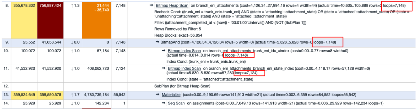
• The construction of bitmap2, which runs 7148 times, is redundant. Because during a short period of time, the constructed bitmap (i.e. rows of attached ENIs) is unlikely to change. It could be put outside the loop, yet it is inside and runs 7148 times in total.
• On average, each execution of the Bitmap Heap Scan node takes 105.888 ms (i.e. construct bitmaps, bitmapAnd, plus the inner-most loop). Because it runs 7148 times, the total execution time of this node alone is 105.888 ms * 7148 = 756,887.424ms = 12 minutes!!
• What’s more, Materialize keeps the Seq Scan result (142234 rows) of assignments table in memory. Even if only the association_id is stored, that’s 20 bytes per row, which translates to 20*142,234 ~=2.8MB in total. Given that 1) we only had 4MB work_mem at the moment and 2) Materialize says it only stored 84k rows rather than all 142k, it’s likely that disk files were used for the query, which could make it even slower.

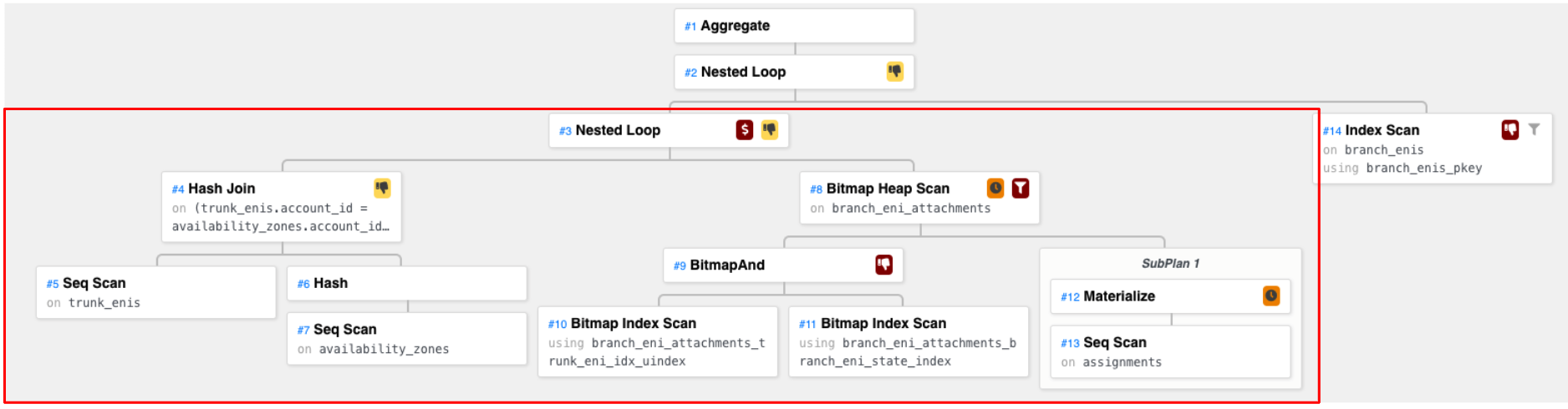
Query Plan Today (and likely before the incident)

As of today, I cannot reproduce the 7-minute query with Bitmap Heap Scan in the prod database even with the same NOT IN query as before. My theory is that the workload changed and the query planner became clever enough to avoid the plan with the expensive Bitmap Heap Scan. The execution plan with the old NOT IN query is like the following, which is likely the plan before the incident since we had never had trouble with it before.

I’ll skip the analysis on this result and list the code-equivalent here directly. Curious readers can do the analysis themselves.

map<string, Az> az_by_account_id;
map<string, Az> az_by_zone_name;
for az in availability_zones
  az_by_account_id[hash(az.account_id)] = az;
  az_by_zone_name[hash(az.zone_name)] = az;

map<string, TrunkEni> trunk_eni_by_id;
for trunck_eni_row in trunk_enis;
  account_id_key = hash(trunk_eni_row.account_id);
  zone_name_key = hash(trunk_eni_row.az);
  if account_id_key in az_by_account_id && zone_name_key in az_by_zone_name
    trunk_eni_by_id[trunk_eni_row.trunk_eni] = trunk_eni_row;

set<string> associations
for assignment_row in assignments
  associations.insert(assignment_row.branch_eni_association)

int count = 0;
for index in branch_eni_attachments_branch_eni_uindex
  attachment_row = get_row_by_index(index)
  if !associations.exists(attachment_row.association_id) && attachment_row.state == "attached" && attachment_row.completed_at < (now() - '00:01:00'::interval)
    if attachment_row.trunk_eni in trunk_eni_by_id
      for branch_eni_index in branch_enis_pkey
        branch_eni_row = get_row_by_index(branch_eni_index)
        if branch_eni_row.branch_eni == attachment_row.branch_eni
          if branch_eni_row.subnet_id == "subnet-1a391a47" && branch_eni_row.last_used < (now() - '01:00:00'::interval)
            count++;
return count

The complexity of this code is O(X + Y + Z + M * N) where

• X: Number of availability zones.
• Y: Number of trunk ENIs
• Z: Number of assignments
• M: Number of branch ENI attachments
• N: Number of branch ENIs

Why the Slow Query Execution Plan?

We now know that the query took 7 minutes to finish on that day because the query plan was bad. Naturally, the next question is, why did the execution suddenly change during the incident? Honestly, the answer is I don’t know. I’m not a DBA and the Postgres planner is a magical black box to me. In theory, the planner uses the system statistics to do some cost analysis and chooses a plan accordingly. It is possible that workload change caused some DB statistics change and in turn caused the planner to yield a bad plan. For example, the size of certain tables might be bigger or smaller than usual.

Nevertheless, one thing I did notice was that the redundant Bitmap Index Scan loop we mentioned above is on an index called branch_eni_attachments_branch_eni_state_index, which is an index on the state column in the branch_eni_attachments table. Though I don’t know what made the planner think that a Bitmap Index Scan should be performed on that index, IMHO, that index on state should not exist in the first place. Because most of the time, the rows have only 2 states – ‘attached’ and ‘unattached’ and both states occupy a large portion of the table. E.g.

> SELECT state, COUNT(*) FROM branch_eni_attachments group by state;
   state    | count
------------+-------
 attached   | 32956
 unattached | 53013
(2 rows)

Because indexes should not be used on columns that return a high percentage of data rows[1], I think this index should be removed. This can also avoid it being used by Bitmap Index Scan in the future.

References

[1] When Should Indexes Be Avoided?
[2] Explaining the unexplainable – part 2
[3] Explaining the unexplainable – part 3